Queue system configuration example

This is a small toy example that shows how different model configurations can be easily defined and simulated when model parameters are defined as reference variables.

The model is a variation of the Queue system example. You should be familiar with the Queue system example before reading about this example.

This example will show how a function can be used to define and simulate a number of different configurations of a model.

This net can be found in
<cpntoolsdir>/Samples/QueueSystem/QueueSystemConfigs.cpn where <cpntoolsdir> is the directory in which CPN Tools is installed.

The net can also be downloaded here.

Model Configurations

It is often necessary to analyze and compare the behavior of different configurations of a model. It is always possible to change the configuration of a model by manually editing declarations, net structure, and/or net inscriptions. However, it can be quite time consuming to make manual changes to a model, particularly if the changes require that a syntax check has to be done for large parts of the model, and/or if many different configurations have to be defined and investigated.

If model parameters are defined as reference variables, then it is possible to use CPN ML functions to automatically define and simulate different configurations of a model.

In the Queue system, there are several model parameters that affect the behavior of the system, including:

1. The distribution of inter-arrival times for jobs.
2. The queuing strategy.
3. The number of servers.
4. The distribution of processing times for servers.

In this example, we will consider model configurations in which the distribution of inter-arrival times and the queuing strategy will not be changed. As for the Queue system example net, the inter-arrival times for jobs is exponentially distributed with a mean inter-arrival time of 100 time units, and the queuing strategy is first-in-first-out (FIFO).

In contrast to the Queue system example net, this example will geared towards investigating model configurations in which the following parameters vary: the number of servers, the average processing time, and the probability distribution of processing times. Each configuration will have either one server with relatively fast processing times, or two servers with slower processing times. And the processing times will be either exponentially distributed or uniformly distributed integers.

Declarations

Many of the declarations for this net are the same as the net for the Queue system. The following declarations are unique for this example, and they are briefly explained below.

colset ProcDist = with DISCRETE | EXP;

globref num_of_servers = 4;
globref avg_proc_time = 360;
globref procdist = EXP;

fun initServers() = (!num_of_servers)`server;

fun genProcTime() = case !procdist of
EXP => expTime(!avg_proc_time)
| DISCRETE =>
discrete (!avg_proc_time – 10,
!avg_proc_time + 10)

fun simulateConfigs(n:int) =
let
fun setOneServer() = (num_of_servers:=1;
avg_proc_time:=90)

fun setTwoServers() = (num_of_servers:=2;
avg_proc_time:=180)
in
procdist := EXP;
setOneServer();
CPN’Replications.nreplications n;
setTwoServers();
CPN’Replications.nreplications n;

procdist := DISCRETE;
setOneServer();
CPN’Replications.nreplications n;
setTwoServers();
CPN’Replications.nreplications n
end

Values from the ProcDist color set will be used to determine the probability distribution for server processing times. The DISCRETE and EXP values represent that the server processing times should be drawn from a discrete uniform distribution and an exponential distribution, respectively.

The reference variables num_of_servers and avg_proc_time will be used to determine the number of servers in the system and the average processing time for a server, respectively. The initial values for these variables are 4 and 360, respectively.

The procdist reference variable will be used to determine the probability distribution of server processing times during a simulation. The initial value of the variable is EXP.

It is important to note that the contents of the reference variables are never changed when transitions occur in the model. The values of these variables should only be changed immediately before a simulation is started.

The initServers function is used to generate a multi-set of server values (from the Server color set shown for the Queue system). The number of server elements in the multi-set is determined by the contents of the num_of_servers reference variable.

The genProcTime function is used to generate server processing times. The contents of the procdist reference variable will determine whether the processing times will be exponentially or uniformly distributed. In either case, the average processing time is determined by the avg_proc_time reference variable.

If the contents of procdist is the value EXP, then the server processing times will be generated by the exponential random variate generator, which is called in the expTime function as defined for the Queue system.

Similarly, if the contents of procdist is the value DISCRETE, then the server processing times will be generated by the the discrete random variate generator, and the values will be drawn from the interval [!avg_proc_time-10, !avg_proc_time+10].

The function simulateConfigs is used to define and simulate a number of different configurations of the model. The function is not used in the model itself. An example of how the function can be used is described below. The functions setOneServer and setTwoServers are used to change the values of the reference variables num_of_servers and avg_proc_time. The first function defines a configuration representing a queuing system with one relatively fast server. The second function determines a configuration with two slower servers. The expressions procdist:=EXP; and procdist:=DISCRETE; in the body of simulateConfigs determine that in some simulations the server processing times should be exponentially distributed, and in other simulations the processing times should be uniformly distributed. The function CPN'Replications.nreplications is a simulator function that is used to execute a given number of simulation replications.

Model

This model contains 3 pages with net structure: System, Arrivals, and Server. The System and Arrivals pages are the same as in the Queue system example.

The Server page for this example is somewhat different than the Server page in the Queue system example, and it looks like this:

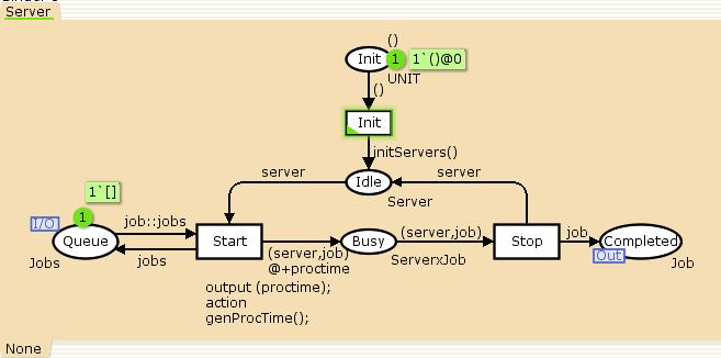
Server page

The Init place and transition are used to initialize the number of servers represented in the system. These nodes are used for technical reasons, as described in the help page for model parameters. The Init transition is only enabled at the beginning of a simulation, and it can only occur once during a simulation. When it occurs, the initServer function is called, and tokens representing servers are added to place Idle. The number of tokens added to the place is determined by the current contents of the num_of_servers reference variable.

The genProcTime function is called in the code segment for the Start transition. The value returned by the function is used to calculate the time stamp for the token that is added to place Busy, and this value represents the amount of time that the server will spend processing the job that has just been removed from the head of the queue of jobs. As described above, the contents of the reference variable procdist determines whether the processing times are drawn from an exponential or discrete uniform distribution.

Monitors

Four monitors have been defined for the model:

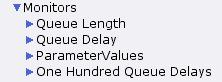
Overview of monitors

The Queue Length monitor is a list length data collector monitor that measures the length of the list on place Queue. This monitor is similar to the List_length_dc_System'Queue_1 monitor described on the help page for Queue System Queue Length.

The Queue Delay monitor is a generic data collector monitor that measures the amount of time that a job spent in a queue. Queue delay is measured each time the Start transition occurs. This monitor is the same as the Queue Delay monitor described on the help page for Queue System Queue Delay.

The ParameterValues monitor is a s|write-in-file monitor. It will update a file once during a simulation when the Init transition on the Server page occurs. The monitor’s observation function is defined to generate a string containing information about the current values of the three reference variables:

fun obs (bindelem) =
“Number of servers: “^(Int.toString(!num_of_servers))^
“\nAverage processing time: “^(Int.toString(!avg_proc_time))^
“\nDistribution of processing times: “^ProcDist.mkstr(!procdist)

The One Hundred Queue Delays monitor is a breakpoint monitor that is defined to stop a simulation after 100 jobs have been removed from the queue. This monitor is similar to the OneHundred_QueueDelays monitor described on the help page for Queue System Miscellaneous Monitors.

Simulating several configurations

Given the simulateConfig function described above, it is possible to automatically simulate the four different configurations defined in the function. The four configurations are:

1. One server with exponentially distributed processing times, and an average processing time of 90.
2. Two servers with exponentially distributed processing times, and an average processing time of 180.
3. One server with uniformly distributed processing times taken from the interval [80..100].
4. Two servers with uniformly distributed processing times taken from the interval [170..190].

Simulations of each of these four configurations can be run by applying the Evaluate ML tool to an auxiliary text containing a CPN ML expression that calls the simulateConfig function. Here is an example of how to run 5 simulations of each of the configurations:

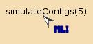
Simulate configurations