What is performance analysis?
Performance is often a central issue in the design, development, and configuration of systems. It is not always enough to know that systems work properly, they must also work effectively. Performance analysis studies are conducted to evaluate existing or planned systems, to compare alternative configurations, or to find an optimal configuration of a system.
Simulation-based performance analysis of a model involves a statistical investigation of output data, the exploration of large data sets, the appropriate visualization of output data, and the verification and validation of simulation experiments. Simulation output is most often random, therefore appropriate statistical techniques must be used both to design and to interpret simulation experiments.
Performance analysis using CPNs must rely on simulation to calculate performance measures for the model. During a simulation of a CPN, the CPN can contain and generate quite a bit of quantitative information about the performance of a system, such as queue length, response time, throughput, etc. This information can be extracted from the model by examining the markings
of places and the occurring binding elements during simulations.
Examples of performance measures that can be calculated by extracting data from markings include:
- Average queue length, where the queue can be represented by
- The individual tokens on a place
- The elements in a list in a list color set
- The elements in a list where the list is one part of a compound color set
- Resource utilization, where busy and idle resources can be represented as
- Tokens on different places, e.g. a Busy place and an Idle place
- Tokens on one place, where the status of a resource is represented as a field in a product color set or record color set.
Examples of performance measures that can be calculated by extracting data from occurring binding elements include:
- End-to-end delay, where one of the variables of the transition is bound to an object, e.g. a packet that has arrived at its final destination. In this case, the departure time for the object will probably have to be included in the information associated with the object.
- Network reliability, where packet loss can be represented as
- A particular transition occurring
- A transition occurring with particular bindings
Calculating performance measures
Performances measures that are calculated via simulation are generally only estimates of the true performance measures. Confidence intervals can be used to indicate how precise estimates of a performance measure are.
The monitoring facilities can be used to extract and save data from CP-nets during simulations. Each performance measure is calculated by a data collector monitor, and each data collector monitor may calculate more than one performance measure of interest. For example, a data collector that measures the length of a queue of packets can calculate both the average length of the queue as well as the maximum length of the queue. The data collector can also calculate the minimum length of the queue, but this may not be an interesting performance measure, particularly if the queue is always empty at the start or end of a simulation.
Timed CP-nets
In many cases, timed CPNs will be used for performance analysis. A timed CPN can model how much time certain activities require, and how much time passes between other activities. In most cases it is insufficient to model the average amount of time that a certain activity takes — it is necessary to include a more precise representation of the timing of the system. The random distribution functions can be used to precisely model time delays.
Consider a system in which new items arrive in the system with exponentially distributed inter-arrival times. Below is an example of a function in which the exponential function is used to create inter-arrival times that are approximately exponentially distributed. The inter-arrival times are only approximately exponentially distributed because the real values that are returned by the exponential function must be converted to integers, since all time delays must be integer values. (Time delay inscriptions can be added as arc inscriptions and transition inscriptions).
fun expTime (mean: int) =
let
val realMean = Real.fromInt mean
val rv = exponential((1.0/realMean))
in
floor (rv+0.5)
end;
This function can then be used when modeling the arrival of new items to a system. A new item is created, i.e. it arrives in the system, when the transition Arrive occurs. The time stamp for the token on place Next determines when the Arrive transition will be enabled, and the expTime function is used to ensure that the inter-arrival times of new items are (approximately) exponentially distributed.

Exponentially distributed inter-arrival times
Workload
When analyzing the performance of a system, one is often interested in
measuring the performance of system when it processes a particular kind of workload. For example, the workload for the Simple Protocol is data packets, and when studying a bank the workload could be customers. With CPNs it is possible to use both fixed workloads, i.e. workloads that are predetermined at the start of a simulation, and dynamic workloads.
In the example net for the Simple Protocol, the workload is fixed, and it is determined by the initial marking for the place Send.
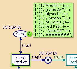
Fixed workload
It is also possible to generate workload on-the-fly during a simulation. In the example below the workload is jobs. The timed token on the place Next determines that a new job will be created periodically, and the inter-arrival times of jobs is exponentially distributed with a mean of 100, as described above.
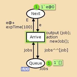
Dynamic workload
Kinds of simulations
Statistical techniques exist for using simulation models to analyze terminating and non-terminating systems.
Terminating simulations
Terminating systems are characterized by having a fixed starting condition and a naturally occurring event that marks the end of the system. An example of a terminating system is a work day that starts at 8 am and ends at 4 pm at a bank. For terminating systems the initial conditions of the system generally affect the desired measures of performance. The purpose of simulating terminating systems is to understand their behavior during a certain period of time, and this is also referred to as studying the transient behavior of the system. Terminating simulations are used to simulate terminating systems. The length of a terminating simulation is determined either by the system itself, if the system is a terminating system, or by the objective of a simulation study. For example, the goal of a performance study may be to analyze the performance of either the entire work day at the bank or only during the time it takes to assist the first 10 customers. The length of a terminating simulation can be determined by a fixed amount of time, e.g. 8 hours, or it can be determined by some condition, e.g. the departure of the tenth customer.
When studying terminating systems,
independent and identically distributed (IID) estimates of performance measures must be collected from a number of independent, terminating simulations. CPN Tools currently provides support for performance analysis using simulation replications of independent, terminating simulations.
Nonterminating simulations
In a non-terminating system, the duration of the system is not finite. The Internet exemplifies a non-terminating system. Non-terminating simulations are used to simulate non-terminating systems. In a non-terminating simulation, there is no event to signal the end of a simulation, and such simulations are typically used to investigate the long-term behavior of a system. Non-terminating simulations must, of course, stop at some point, and it is a non-trivial problem to determine the proper duration of a non-terminating simulation. If the behavior of the system becomes fairly stable at some point, then there are techniques for analyzing the steady-state behavior of the system using non-terminating simulations. When analyzing steady-state behavior using non-terminating simulations, it is often useful to be able to specify a warm-up period in which data is not collected because the model has not yet reached a steady state. Determining when, or if, a model reaches steady state is also a complicated issue.
Note that CPN Tools does not currently provide high-level support for performance analysis using warm-up periods or non-terminating simulations.
Experimental design
After a model has been created and validated, there are a number of decisions that need to be made before a study can proceed. Experimental design is concerned with determining which scenarios are going to be simulated and how each of the scenarios will be simulated in a simulation study. For each scenario in a simulation study one needs to decide how many simulations will be run, how long the simulations will be, and how each scenario will be initialized. Both the length of a simulation and the number of replications run can have a significant impact on the performance measure estimates. Making arbitrary, unsystematic or improper decisions is a waste of time, and the simulation study may fail to produce useful results.
Help topics for performance analysis
- Monitors
- Create a monitor
- Data types for monitored subnets
- Edit a monitor
- Errors in monitors
- Monitoring functions
- Monitor template code
- Breakpoint monitors
- Breakpoint monitoring functions
- Data collector monitors
- Data Collector Monitoring Functions
- User-defined monitors
- User-defined monitoring functions
- Write-in-file monitors
- Write-in-file monitoring functions
- Monitor index entries
- Known limitations of monitors
- Random distribution functions
- Bernoulli
- Beta
- Binomial
- Chi-square
- Discrete
- Erlang
- Exponential
- Gamma
- Normal
- Poisson
- Rayleigh
- Student
- Uniform
- Weibull
- Performance output
- Performance options functions
- Output management functions
- Output management
- Independent and identically distributed values
- Data collector functions
- Calculating statistics
Example nets for performance analysis:
Known limitations
Performance output can contain statistics for data collectors that are disabled.
Related pages
Tasks in CPN Tools, Data collector monitors, Simulation replications, Model parameters, Time attributes in tokens
You must be logged in to post a comment.